Lesson 4 - Equilibrium and Coarsegraining

In Lesson 1, we noted that as systems approach equlibrium, the energy and matter in the system tends to “spread out”. In this lesson, we will use coarse-graining as a way to study the approach to an equilibrium state. In this lesson we focus on the spreading out of matter in the billiard balls model; in later lessons we return to study the spreading out of energy.

An Expanding Gas

This animation shows a billiard ball model initialized with all of the particles on one half of the box.

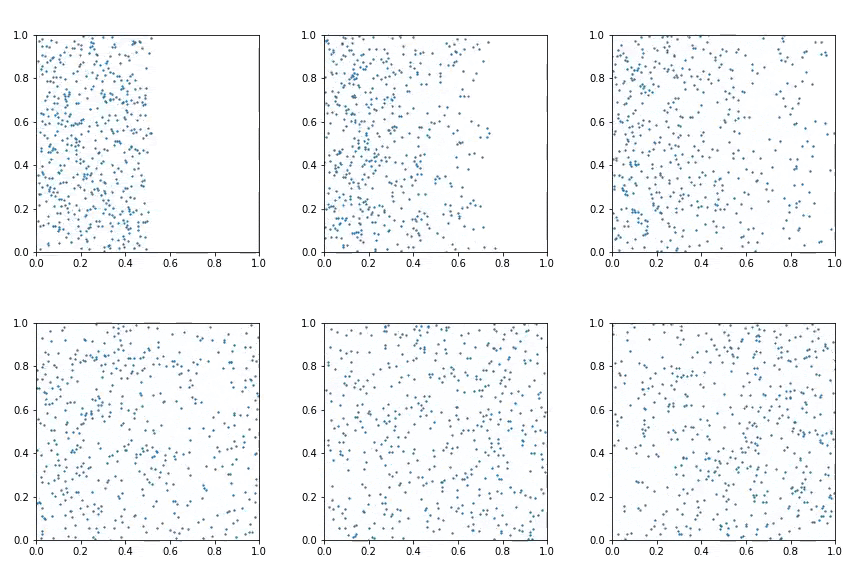
Intuitively, it’s clear that in equilibrium, the particles are spread out through the whole box. How can we quantify this though? What makes a configuration with the particles spread out over the whole table different from one where they are localized on one half?

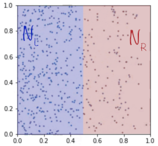
We can make a clearer definition of equilbrium by defining macroscopic coarse-grained variables. As a simple example, we can choose the number of atoms on the left hand side of the box \(N_L\) and the number of atoms on the right hand side of the box \(N_R\) as macroscopic variables sensitive to the spreading out of the atoms:

The values of theses coarse-grained variables will depend on time as the particles spread out and bounce around. Shown below is \(N_L(t)\) as the simulation evolves.

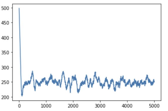
The plot starts at large values, corresponding to most particles being found on the left hand side, than rapidly decreases as the particles expand. After a few hundred time steps, it begins fluctuating around a relatively constant mean value, where approximately half the particles are on the left hand side. This gives us a much clearer definition of equilbrium – although the microscopic configuration changes continously and our macroscopic coarse-grained variables continue to fluctuate, equilibrium can be said roughly to occur when all of the coarse-grained variables are fluctuating around their mean values. Although it might not be obvious, this statement is surprising robust to the choice of macroscopic coarses-grained variables – for example, we could have split the box into 4 quadrants to measure the density instead, and still found roughly the same results.

You might be worried that “fluctuating around their mean values” is not a very exact description of equilibrium, and you would be right to be concerned! Another approach to defining equilibrium is to say that in equilibrium, the distribution of any coarse-grained variable converges. What does that mean? Consider three different time regions in the above plot:

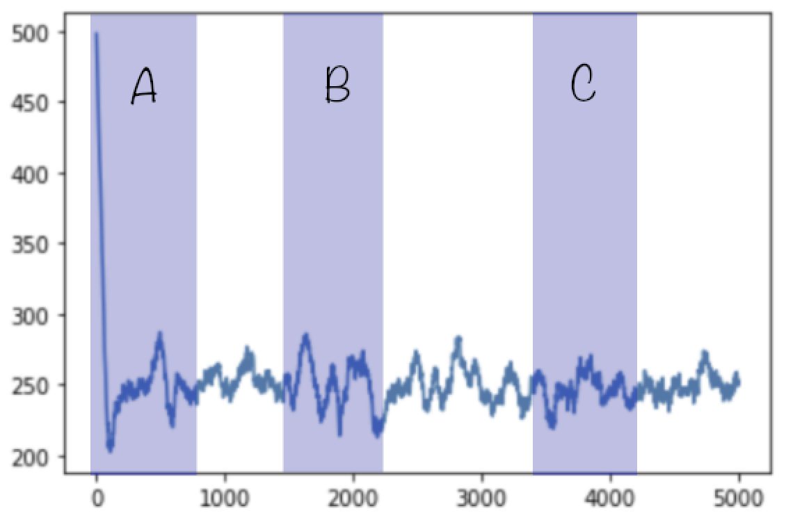
If we plot the histogram of \(N_L\) in the time region A, we will get quite different results than in region B or C, because of the initial condition with a much larger than typical number of particles on the left hand side:

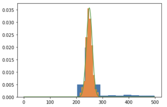
The orange distribution shows the distribution in time window B, which has reached a near-Gaussian shape, while the blue distribution shows the distribution in time window A with a large tail toward \(N_L = 500\). At C, this distribution will be little changed from B, so we say that the system has indeed reached equilibrium. Pragmatically, to identify the onset of equilibrium in this way, some care is required in choosing large enough time windows to get a good distribution, but not so large that you wash out the initial out of equilibrium conditions!

In the pre-class work and in class activities you will reproduce some of these results and probe them further, in particular connecting the size of fluctuations in equilibrium to what we learned in Lesson 2 about the central limit theorem and fluctuations in random walks.

Universality of Equilibrium

A crucial aspect of equilibrium is its universality. We could run our simulation with many different microscopic configurations of the particles in different initial conditions, and we find nonetheless the same equilbrium mean values of the macroscopic varibles, and indeed the same distribution of fluctuations in equilibrium. It does not matter if we start all the particles on the left hand side, the right hand side, all in the center, or in an evenly spaced grid all moving toward the center… in all these cases, the equilibrium properties are the same¹. The approach to equilibrium may be follow a different path or take longer or shorter, but the equilibrium distributions that will be reached are unchanged as long as the number of particles and total initial energy of the particles is unchanged! This is the miracle that allows statistical mechanics to make firm predictions about the world, despite the impossible nature of trying to measure or control the detailed initial microscopic conditions of any macroscopic system.